R - Cultivated crop maps in Rio Grande do Sul, Brazil
Welcome. In this post, I am going to show you how you may create maps of cultivated crops in Rio Grande do Sul state, Brazil.
Generate crop cultivated maps
Crop plantation area from IBGE
Loading the packages
library(readxl)
library(tidyverse)
library(geobr)
library(patchwork)
URL link of data from IBGE on GitHub https://github.com/luanpott10/Class
You will nedd the raw file https://raw.githubusercontent.com/luanpott10/Class/main/tabela1612_1.csv
Load the data and data wrangling
The data downloaded from IBGE there are metadata in the 4 first lines that are not intrest for us skip = 4.
Also, there are info in the last rows, for that we select the 497 municipalities data[1:497,].
Furthermore, the rows (cities) without crop planted, IBGE used “-” or “…” instead input 0, then we have used case_when function.
data <- read_csv('https://raw.githubusercontent.com/luanpott10/Class/main/tabela1612_1.csv', skip = 4)
data <- data[1:497,]

colnames(data) <- c("code","city","rice","corn","soybean")

data <- data |>
  mutate(rice_crop = case_when(rice == "..." | rice == "-" ~ 0,
                                TRUE ~ as.double(rice))) |>
  mutate(corn_crop = case_when(corn == "..." | corn == "-" ~ 0,
                                TRUE ~ as.double(corn))) |>
  mutate(soybean_crop = case_when(soybean == "..." | soybean == "-" ~ 0,
                                TRUE ~ as.double(soybean)))

data <- data |> select(code,city,rice_crop,corn_crop,soybean_crop)
Dataset of geobr package from municipalities of Rio Grande do Sul state
cities_RS <- read_municipality(code_muni = "RS", year= 2020)Ggplot of the cities
ggplot()+
  geom_sf(data=cities_RS)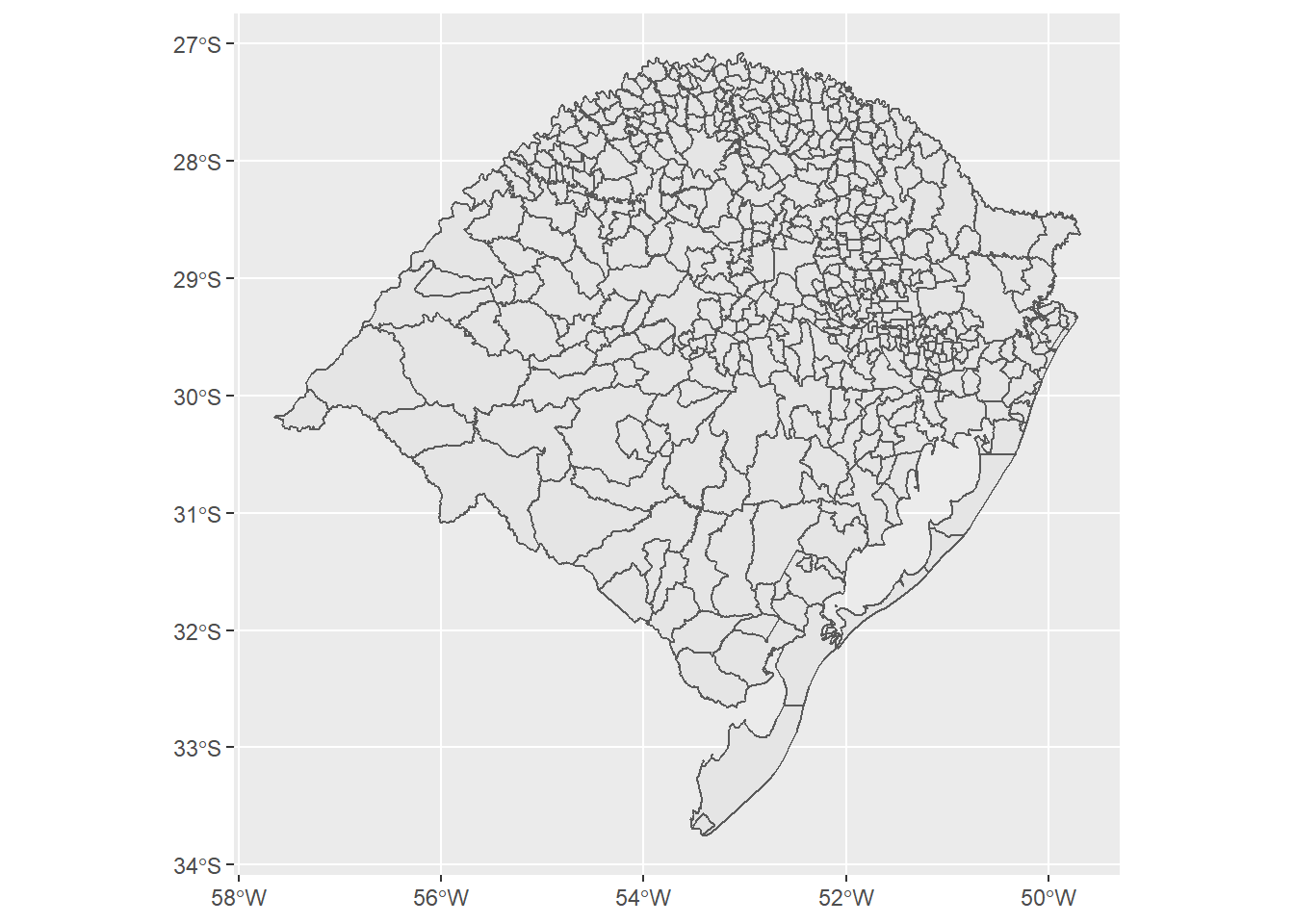
Joining the IBGE data and the sf object
cities_RS$code_muni <- as.character(cities_RS$code_muni)
data_x <- left_join(cities_RS,data,by= c("code_muni"="code"))
Palettes
pal_soybean <- c('#252525','#ccece6','#99d8c9','#66c2a4','#41ae76','#238b45','#006d2c','#00441b')
pal_corn <- c('#252525','#f7ffa8','#EFFD5F','#FCE205','#FCD12A','#FFC30B','#F9A602','#c48302')
pal_rice <- c('#252525','#caebfc','#9ecae1','#6baed6','#4292c6','#2171b5','#084594','#082954')
Soybean map
(soybean_map <-
  ggplot()+
    geom_sf(data=data_x,aes(fill=soybean_crop))+
    theme_minimal()+
    scale_fill_gradientn(colours=pal_soybean,
                       limits = c(0,150000),
                       na.value='#252525')+
    labs(x= "Longitude", y = "Latitude", title = "Soybean")+
    guides(fill=guide_colorbar(title="Crop area (ha)",barwidth = 1,barheight = 4,
                             frame.colour = "black"))+
    theme(legend.position = c(0.17, 0.2),
        panel.border = element_rect(color="Black", fill = NA),
        panel.background = element_rect(fill = "#f2f2f2"),
        panel.grid.major = element_blank(),
        panel.grid.minor = element_blank(),
        axis.title.x = element_text(family = "serif",
                                    colour = "#000000",size = 22.0),
        axis.text.x = element_text(family = "serif",
                                   colour = "#000000",size = 18.0),
        axis.title.y = element_text(family = "serif",
                                    colour = "#000000",size = 22.0),
        axis.text.y = element_text(family = "serif",
                                   colour = "#000000",size = 18.0),
        legend.title = element_text(family = "serif",
                                    colour = '#000000',size = 12.0),
        legend.text = element_text(family = "serif",
                                   colour = '#000000',size = 12.0),
        legend.background = element_rect(fill="#f2f2f2",
                                  linetype="dashed",
                                  colour ="#f2f2f2")))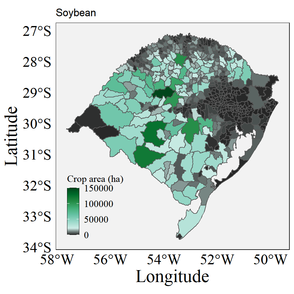
Corn map
(corn_map <-
  ggplot()+
    geom_sf(data=data_x,aes(fill=corn_crop))+
    theme_minimal()+
    scale_fill_gradientn(colours=pal_corn,
                       limits = c(0,15000),
                       na.value='#252525')+
    labs(x= "Longitude", y = "Latitude", title = "Corn")+
    guides(fill=guide_colorbar(title="Crop area (ha)",barwidth = 1,barheight = 4,
                             frame.colour = "black"))+
    theme(legend.position = c(0.17, 0.2),
        panel.border = element_rect(color="Black", fill = NA),
        panel.background = element_rect(fill = "#f2f2f2"),
        panel.grid.major = element_blank(),
        panel.grid.minor = element_blank(),
        axis.title.x = element_text(family = "serif",
                                    colour = "#000000",size = 22.0),
        axis.text.x = element_text(family = "serif",
                                   colour = "#000000",size = 18.0),
        axis.title.y = element_text(family = "serif",
                                    colour = "#000000",size = 22.0),
        axis.text.y = element_text(family = "serif",
                                   colour = "#000000",size = 18.0),
        legend.title = element_text(family = "serif",
                                    colour = '#000000',size = 12.0),
        legend.text = element_text(family = "serif",
                                   colour = '#000000',size = 12.0),
        legend.background = element_rect(fill="#f2f2f2",
                                  linetype="dashed",
                                  colour ="#f2f2f2")))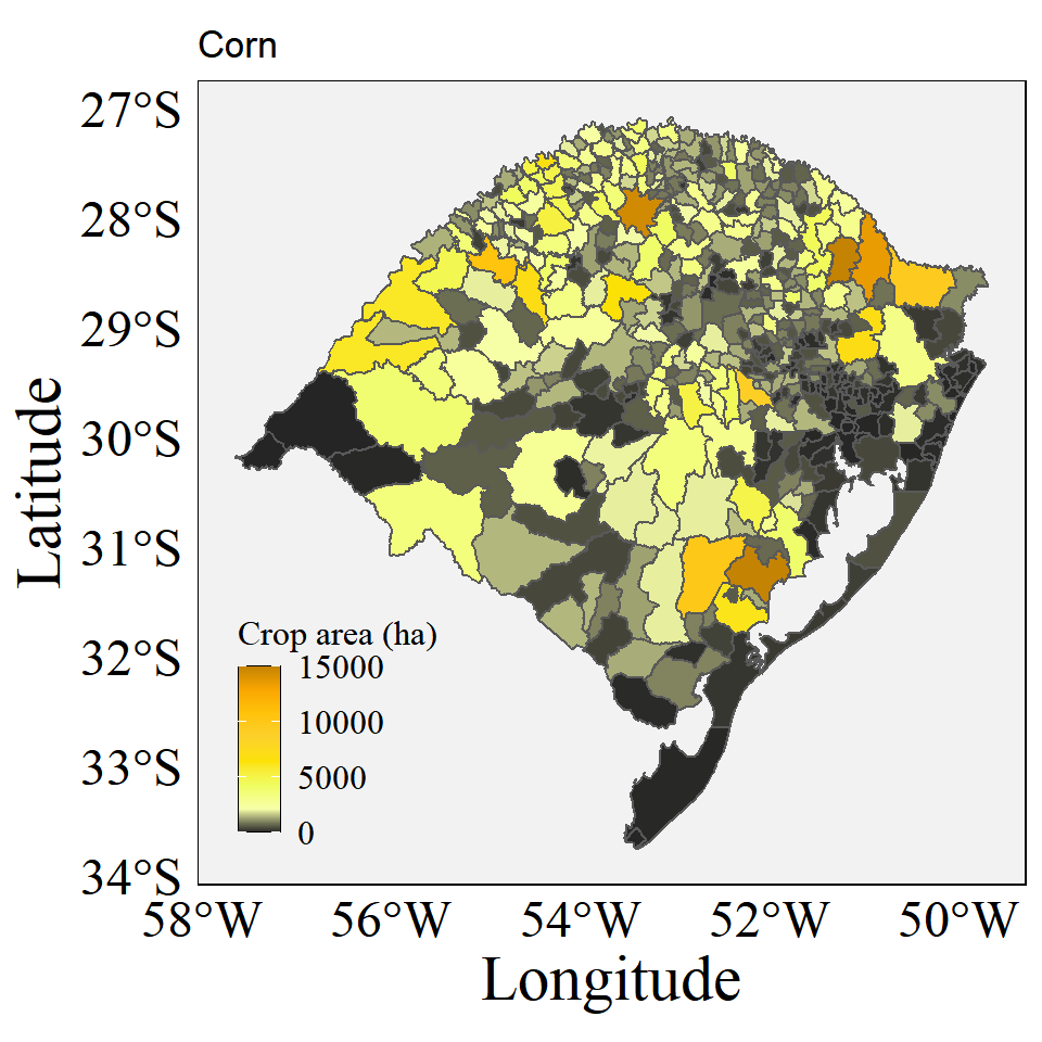
Rice map
(rice_map <-
  ggplot()+
    geom_sf(data=data_x,aes(fill=rice_crop))+
    theme_minimal()+
    scale_fill_gradientn(colours=pal_rice,
                       limits = c(0,75000),
                       na.value='#252525')+
    labs(x= "Longitude", y = "Latitude", title = "Rice")+
    guides(fill=guide_colorbar(title="Crop area (ha)",barwidth = 1,barheight = 4,
                             frame.colour = "black"))+
    theme(legend.position = c(0.17, 0.2),
        panel.border = element_rect(color="Black", fill = NA),
        panel.background = element_rect(fill = "#f2f2f2"),
        panel.grid.major = element_blank(),
        panel.grid.minor = element_blank(),
        axis.title.x = element_text(family = "serif",
                                    colour = "#000000",size = 22.0),
        axis.text.x = element_text(family = "serif",
                                   colour = "#000000",size = 18.0),
        axis.title.y = element_text(family = "serif",
                                    colour = "#000000",size = 22.0),
        axis.text.y = element_text(family = "serif",
                                   colour = "#000000",size = 18.0),
        legend.title = element_text(family = "serif",
                                    colour = '#000000',size = 12.0),
        legend.text = element_text(family = "serif",
                                   colour = '#000000',size = 12.0),
        legend.background = element_rect(fill="#f2f2f2",
                                  linetype="dashed",
                                  colour ="#f2f2f2")))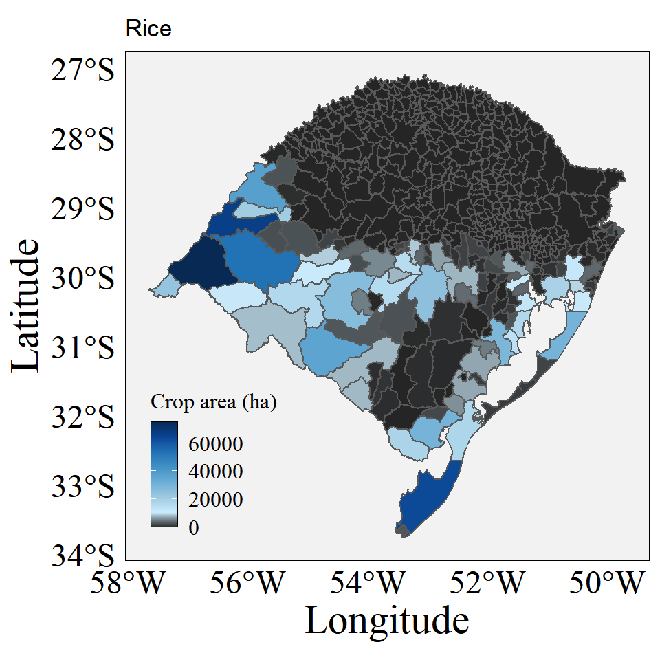
Crop maps
soybean_map + corn_map + rice_map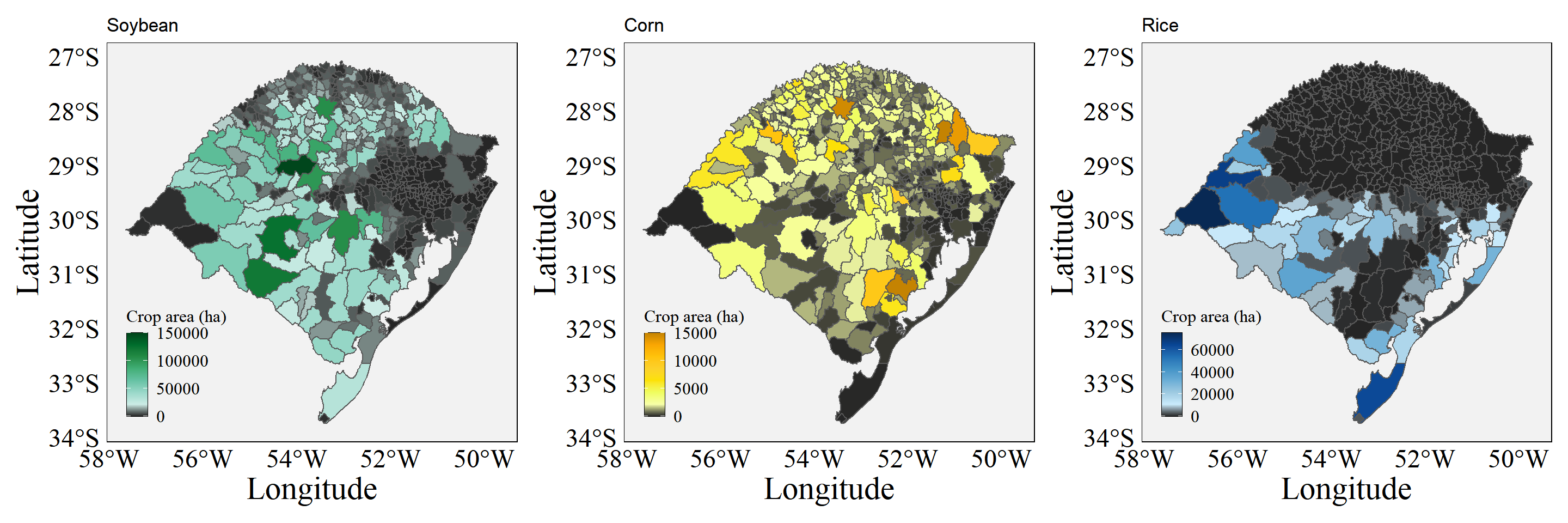
Luan Pierre Pott
PhD student in Agricultural Engineering
My research interests include digital agriculture, remote sensing, crop modeling and machine learning