R - Data visualization, linear regression and logistic regression
Welcome. In this post, I am going to show you how you may create point maps, linear regression and logistic regression utilizing R base tools and tidymodels workflow.
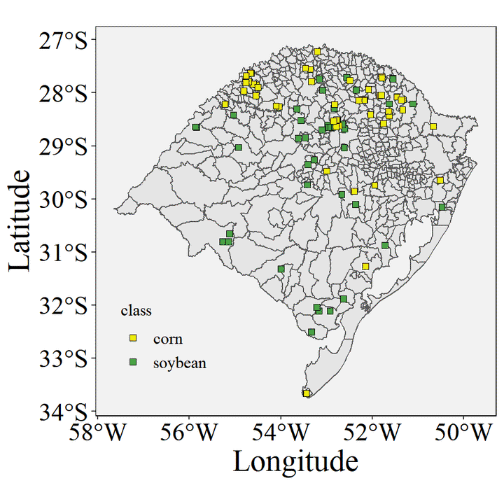 Image credit: Pott L.P.
Data visualization, linear regression and logistic regression
Crop data collection - ground truth and remote sensing
Loading the packages
library(tidyverse)
library(tidymodels)
library(sf)
library(geobr)
URL link of data from data collection and remote sensing on GitHub https://github.com/luanpott10/Class
You will need the raw file https://raw.githubusercontent.com/luanpott10/Class/main/data_crops.csv
Loading the data
data <- read.csv("https://raw.githubusercontent.com/luanpott10/Class/main/data_crops.csv")Plot the data in the map
cities_RS <- read_municipality(code_muni = "RS", year= 2020)

ggplot()+
  geom_sf(data=cities_RS)+
  geom_point(data=data,aes(x=longitude,y=latitude,fill=class),shape=22,size=2)+
  labs(x= "Longitude", y = "Latitude")+
  scale_fill_manual(values = c("#eded0c", "#49a345"))+
  theme(legend.position = c(0.17, 0.2),
        panel.border = element_rect(color="Black", fill = NA),
        panel.background = element_rect(fill = "#f2f2f2"),
        panel.grid.major = element_blank(),
        panel.grid.minor = element_blank(),
        axis.title.x = element_text(family = "serif",
                                    colour = "#000000",size = 22.0),
        axis.text.x = element_text(family = "serif",
                                   colour = "#000000",size = 18.0),
        axis.title.y = element_text(family = "serif",
                                    colour = "#000000",size = 22.0),
        axis.text.y = element_text(family = "serif",
                                   colour = "#000000",size = 18.0),
        legend.title = element_text(family = "serif",
                                    colour = '#000000',size = 12.0),
        legend.text = element_text(family = "serif",
                                   colour = '#000000',size = 12.0),
        legend.background = element_rect(fill="#f2f2f2",
                                  linetype="dashed",
                                  colour ="#f2f2f2"))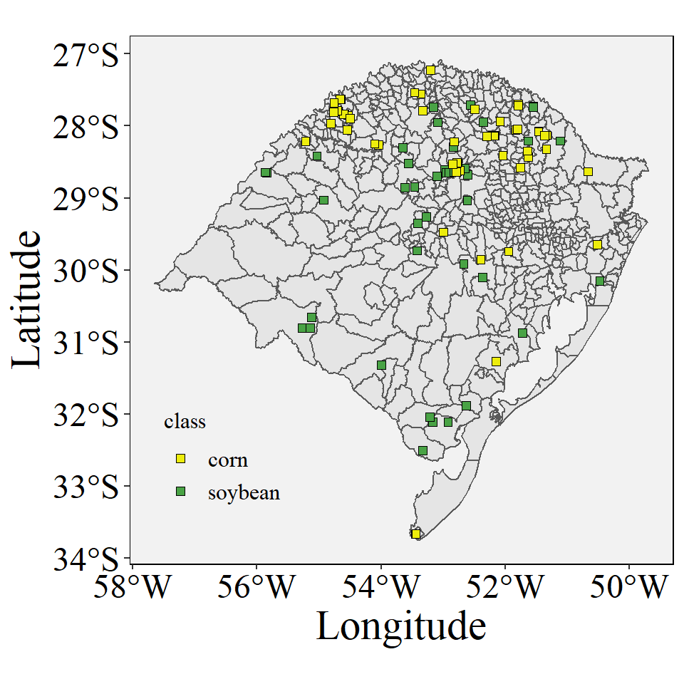
Plot the data variables - continuous x continuous
ggplot(data=data,aes(x=b3_GCVI,y=b4_GCVI))+
  geom_point(aes(fill=class),shape=22,size=2)+
  scale_fill_manual(values = c("#eded0c", "#49a345"))+

  stat_smooth(formula = y~x, method="lm", se=FALSE,color="black", linetype='dashed')+

  theme(panel.border = element_rect(color="Black", fill = NA),
        panel.background = element_rect(fill = "#f2f2f2"),
        panel.grid.major = element_blank(),
        panel.grid.minor = element_blank(),
        axis.title.x = element_text(family = "serif",
                                    colour = "#000000",size = 22.0),
        axis.text.x = element_text(family = "serif",
                                   colour = "#000000",size = 18.0),
        axis.title.y = element_text(family = "serif",
                                    colour = "#000000",size = 22.0),
        axis.text.y = element_text(family = "serif",
                                   colour = "#000000",size = 18.0),
        legend.title = element_text(family = "serif",
                                    colour = '#000000',size = 12.0),
        legend.text = element_text(family = "serif",
                                   colour = '#000000',size = 12.0),
        legend.background = element_rect(fill="#f2f2f2",
                                  linetype="dashed",
                                  colour ="#f2f2f2"))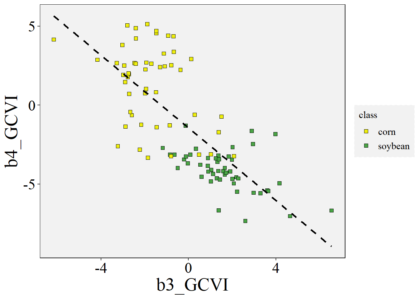
Linear regression
lm_fit_x <- lm(b3_GCVI ~ b4_GCVI, data = data)
summary(lm_fit_x)
##
## Call:
## lm(formula = b3_GCVI ~ b4_GCVI, data = data)
##
## Residuals:
##     Min      1Q  Median      3Q     Max
## -3.7924 -0.9983 -0.0018  0.9525  3.9586
##
## Coefficients:
##             Estimate Std. Error t value Pr(>|t|)
## (Intercept) -0.73701    0.15933  -4.626 1.14e-05 ***
## b4_GCVI     -0.49793    0.04352 -11.440  < 2e-16 ***
## ---
## Signif. codes:  0 '***' 0.001 '**' 0.01 '*' 0.05 '.' 0.1 ' ' 1
##
## Residual standard error: 1.475 on 98 degrees of freedom
## Multiple R-squared:  0.5718, Adjusted R-squared:  0.5675
## F-statistic: 130.9 on 1 and 98 DF,  p-value: < 2.2e-16
Linear regression by tidymodels workflow
Creating a parsnip specification for a linear regression model
lm_model <- linear_reg() |>
            set_engine('lm') |>
            set_mode('regression')
Fitting the model supplying a formula expression and the data
lm_fit <- lm_model %>%
          fit(b3_GCVI ~ b4_GCVI, data = data)
Summary of the model
lm_fit |>
  pluck("fit") |>
  summary()
##
## Call:
## stats::lm(formula = b3_GCVI ~ b4_GCVI, data = data)
##
## Residuals:
##     Min      1Q  Median      3Q     Max
## -3.7924 -0.9983 -0.0018  0.9525  3.9586
##
## Coefficients:
##             Estimate Std. Error t value Pr(>|t|)
## (Intercept) -0.73701    0.15933  -4.626 1.14e-05 ***
## b4_GCVI     -0.49793    0.04352 -11.440  < 2e-16 ***
## ---
## Signif. codes:  0 '***' 0.001 '**' 0.01 '*' 0.05 '.' 0.1 ' ' 1
##
## Residual standard error: 1.475 on 98 degrees of freedom
## Multiple R-squared:  0.5718, Adjusted R-squared:  0.5675
## F-statistic: 130.9 on 1 and 98 DF,  p-value: < 2.2e-16
# Also you can use
lm_fit$fit |> summary()
##
## Call:
## stats::lm(formula = b3_GCVI ~ b4_GCVI, data = data)
##
## Residuals:
##     Min      1Q  Median      3Q     Max
## -3.7924 -0.9983 -0.0018  0.9525  3.9586
##
## Coefficients:
##             Estimate Std. Error t value Pr(>|t|)
## (Intercept) -0.73701    0.15933  -4.626 1.14e-05 ***
## b4_GCVI     -0.49793    0.04352 -11.440  < 2e-16 ***
## ---
## Signif. codes:  0 '***' 0.001 '**' 0.01 '*' 0.05 '.' 0.1 ' ' 1
##
## Residual standard error: 1.475 on 98 degrees of freedom
## Multiple R-squared:  0.5718, Adjusted R-squared:  0.5675
## F-statistic: 130.9 on 1 and 98 DF,  p-value: < 2.2e-16
Parameter estimates of a the lm object
tidy(lm_fit)
## # A tibble: 2 x 5
##   term        estimate std.error statistic  p.value
##   <chr>          <dbl>     <dbl>     <dbl>    <dbl>
## 1 (Intercept)   -0.737    0.159      -4.63 1.14e- 5
## 2 b4_GCVI       -0.498    0.0435    -11.4  9.39e-20
Extract the model statistics
glance(lm_fit)
## # A tibble: 1 x 12
##   r.squared adj.r.squared sigma statistic  p.value    df logLik   AIC   BIC
##       <dbl>         <dbl> <dbl>     <dbl>    <dbl> <dbl>  <dbl> <dbl> <dbl>
## 1     0.572         0.567  1.47      131. 9.39e-20     1  -180.  365.  373.
## # ... with 3 more variables: deviance <dbl>, df.residual <int>, nobs <int>
Plot the data variables - categorical x continuous
data <- data |> mutate(target = case_when(class == "corn" ~ 0,
                                          class == "soybean" ~ 1))

ggplot(data=data, aes(y=target,x=b4_GCVI))+
  geom_point(aes(fill=as.factor(target)),shape=22,size=2) +
  scale_fill_manual(values = c("#eded0c", "#49a345"))+
  scale_y_continuous(breaks=c(0,1),
                   labels=c("0","1"),
                   limits=c(0,1))+

  stat_smooth(formula = y~x, method="glm", se=FALSE, method.args = list(family=binomial),
              color="black", linetype='dashed')+
  labs(x= "b4_GCVI", y = "Class",fill="Class")+

  theme(legend.position = c(0.17, 0.2),
        panel.border = element_rect(color="Black", fill = NA),
        panel.background = element_rect(fill = "#f2f2f2"),
        panel.grid.major = element_blank(),
        panel.grid.minor = element_blank(),
        axis.title.x = element_text(family = "serif",
                                    colour = "#000000",size = 22.0),
        axis.text.x = element_text(family = "serif",
                                   colour = "#000000",size = 18.0),
        axis.title.y = element_text(family = "serif",
                                    colour = "#000000",size = 22.0),
        axis.text.y = element_text(family = "serif",
                                   colour = "#000000",size = 18.0),
        legend.title = element_text(family = "serif",
                                    colour = '#000000',size = 12.0),
        legend.text = element_text(family = "serif",
                                   colour = '#000000',size = 12.0),
        legend.background = element_rect(fill="#f2f2f2",
                                  linetype="dashed",
                                  colour ="#f2f2f2"))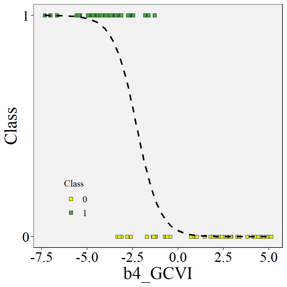
Logistic regression
lg_fit_x <- glm(as.factor(class) ~ b4_GCVI, family="binomial", data=data)
summary(lg_fit_x)
##
## Call:
## glm(formula = as.factor(class) ~ b4_GCVI, family = "binomial",
##     data = data)
##
## Deviance Residuals:
##      Min        1Q    Median        3Q       Max
## -1.91207  -0.04298   0.01134   0.32227   1.86651
##
## Coefficients:
##             Estimate Std. Error z value Pr(>|z|)
## (Intercept)  -3.5734     1.1155  -3.203  0.00136 **
## b4_GCVI      -1.5677     0.3778  -4.150 3.33e-05 ***
## ---
## Signif. codes:  0 '***' 0.001 '**' 0.01 '*' 0.05 '.' 0.1 ' ' 1
##
## (Dispersion parameter for binomial family taken to be 1)
##
##     Null deviance: 138.629  on 99  degrees of freedom
## Residual deviance:  42.379  on 98  degrees of freedom
## AIC: 46.379
##
## Number of Fisher Scoring iterations: 7
Logistic regression by tidymodels workflow
Creating a parsnip specification for a logistic regression model
lg_model <- logistic_reg() |>
        set_engine("glm") |>
        set_mode("classification")
Fitting the model supplying a formula expression and the data
lg_fit <- lg_model |>
          fit(as.factor(class) ~ b4_GCVI, data = data)
Summary of the model
lg_fit |>
  pluck("fit") |>
  summary()
##
## Call:
## stats::glm(formula = as.factor(class) ~ b4_GCVI, family = stats::binomial,
##     data = data)
##
## Deviance Residuals:
##      Min        1Q    Median        3Q       Max
## -1.91207  -0.04298   0.01134   0.32227   1.86651
##
## Coefficients:
##             Estimate Std. Error z value Pr(>|z|)
## (Intercept)  -3.5734     1.1155  -3.203  0.00136 **
## b4_GCVI      -1.5677     0.3778  -4.150 3.33e-05 ***
## ---
## Signif. codes:  0 '***' 0.001 '**' 0.01 '*' 0.05 '.' 0.1 ' ' 1
##
## (Dispersion parameter for binomial family taken to be 1)
##
##     Null deviance: 138.629  on 99  degrees of freedom
## Residual deviance:  42.379  on 98  degrees of freedom
## AIC: 46.379
##
## Number of Fisher Scoring iterations: 7
# Also you can use
lg_fit$fit |> summary()
##
## Call:
## stats::glm(formula = as.factor(class) ~ b4_GCVI, family = stats::binomial,
##     data = data)
##
## Deviance Residuals:
##      Min        1Q    Median        3Q       Max
## -1.91207  -0.04298   0.01134   0.32227   1.86651
##
## Coefficients:
##             Estimate Std. Error z value Pr(>|z|)
## (Intercept)  -3.5734     1.1155  -3.203  0.00136 **
## b4_GCVI      -1.5677     0.3778  -4.150 3.33e-05 ***
## ---
## Signif. codes:  0 '***' 0.001 '**' 0.01 '*' 0.05 '.' 0.1 ' ' 1
##
## (Dispersion parameter for binomial family taken to be 1)
##
##     Null deviance: 138.629  on 99  degrees of freedom
## Residual deviance:  42.379  on 98  degrees of freedom
## AIC: 46.379
##
## Number of Fisher Scoring iterations: 7
Parameter estimates of a the lm object
tidy(lg_fit)
## # A tibble: 2 x 5
##   term        estimate std.error statistic   p.value
##   <chr>          <dbl>     <dbl>     <dbl>     <dbl>
## 1 (Intercept)    -3.57     1.12      -3.20 0.00136
## 2 b4_GCVI        -1.57     0.378     -4.15 0.0000333
Extract the model statistics
glance(lg_fit)
## # A tibble: 1 x 8
##   null.deviance df.null logLik   AIC   BIC deviance df.residual  nobs
##           <dbl>   <int>  <dbl> <dbl> <dbl>    <dbl>       <int> <int>
## 1 139. 99 -21.2 46.4 51.6 42.4 98 100Luan Pierre Pott
PhD student in Agricultural Engineering
My research interests include digital agriculture, remote sensing, crop modeling and machine learning